DEX Arbitrage, Mathematical Optimisations & Me
How to efficiently maximise arbitrage profit over a set of exchanges via Convex Optimisation
If you’re a scholar of MEV, understanding how to maximise arbitrage profit is something you should be interested in.
Lucky for you that’s what we’ll be diving into today.
By far the largest form of MEV on-chain is arbitrage. The concept is simple, find price differences between exchanges on given tokens, execute a trade, pocket some profit and in the process bring the token prices on the exchanges back in line with each other.
While the concept is simple, finding the highest yielding arbitrage across a large set of exchanges and tokens can be difficult.
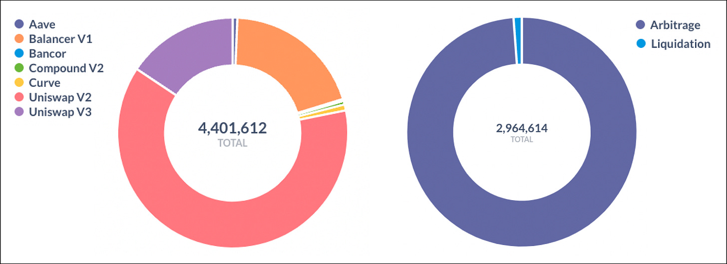
When finding an optimal arbitrage you’re racing against the block time of the chain and there are lots of moving parts. New transactions in the mempool, changing reference prices on centralised exchanges etc.
Lucky for us finding this optimal arbitrage has been found to be a “convex optimsation” problem for Constant Function Market Makers (CFMMs) like Uniswap, Sushiswap, Balancer etc.
What this means will be the subject of this article but to give you a taster it means that we can efficiently solve the arbitrage problem to global optimality.
Or in plain English, we have a formula that can efficiently find the set of trades that maximises arbitrage profit across a set of CFMMs.
Mathematical Optimisations
Convex optimisations are a subfield of mathematical optimisations.
If we want to learn about convex optimisations a good place to start is gaining a high-level understanding of what a mathematical optimisation is.
Mathematical optimisation is the selection of a best element, with regard to some criterion, from some set of available alternatives
So what does this actually mean, let’s focus on the most common use case which is using mathematical optimisations when handling min/max problems.
Min/Max problems are problems that minimise or maximise an “objective function” given some “constraints” on the input values of that function.
Note that constraints can come in the form of inequality constraints (x^2 + y^2 >= 1) or equality constraints (x^2 + y^2 = 1).
For example, given a budget buy as many pieces of fruit from the supermarket as possible where each fruit has a different price. Our constraints could be we can buy no more than 5 bananas (b <= 5 inequality constraint) and that we must buy exactly one orange (o = 1 equality constraint).
Now let’s look at a more complex example and the notation that would be used to represent the problem. I will also provide an alternative way to view it which may be more intuitive for someone from a programming background.
Constrained Optimisation Example
You are asked to maximise the objective function f( x, y ) where,
f( x, y ) = x^2 * y with the constraint
x^2 + y^2 = 1Let’s start with the constraint, the constraint provides us with a set of viable x & y values.
For example, when x = 1 & y = 1, x^2 + y^2 = 2 which is not 1. Therefore it does not meet the constraint and is not a valid x, y position.
When x = 0.70710678118 & y = 0.70710678118, x^2 + y^2 = 1 which is equal to 1. Therefore these x, y co-ordinates do meet the constraint and are valid.
This same objective function and constraints can be represented in the form of a function in python. Our objective is to maximise what the function returns.
The function objective_function( x, y ) and is equivalent to f( x, y ). For the constraint, I have raised an exception if it isn’t met rather than using an indicator/penalty function.
This problem can be viewed graphically with 3 axes, one for x, one for y and one for the returned result f( x, y ).
Above is a 3-dimensional graph that represents this problem. The red circle represents all the x, y coordinates that satisfy the constraint
x^2 + y^2 = 1Another way to visualise this graph is to imagine drawing the x & y axes on the floor in a large playground using some chalk.
Given x, y coordinates, we can walk to that position in the playground and at that location a value, f( x, y ), will be returned to us.
The returned value is the objective function we’re trying to maximise. Its value will represent some height above or below the floor. Therefore the height above/below the ground represents our third axis f( x, y ).
If we had the ability to place a floating tennis ball above/below the ground based on the returned f( x, y ) we could plot out the 3-dimensional graph.
We would simply walk around the playground note the x & y position and place our tennis ball some point above or below the ground.
If done at every coordinate this network of floating tennis balls would match the 3-dimensional graph we see in the images above.
The maximisation question can then be thought of as given a set of tennis balls placed above / below the ground at all playground coordinates (x, y) where x^2 + y^2 = 1 find the tennis ball that is the highest above the ground.
Framing an Optimisation Problem
The purpose of this example is it shows us how an optimisation problem is framed.
We have some objective function which is the thing we want to minimise/maximise and a set of constraints. The importance of this will become apparent when we look at a real-world arbitrage.
This is all the context we need for the rest of this article however if you are interested in learning more about this specific problem there are a set of videos that describe the solution. Feel free to come back at the end and run through them to help aid your understanding.
Now let’s move on to the optimisation specific to CFMM arbitrage, convex optimisation.
Convex Optimisation
First, let’s start by looking at what makes our CFMM arbitrage optimisation problem convex. We’ll be dealing with a lot of what we have already encountered namely the objective function and constraints.
The objective function must be convex.
The equality function can be linear, you may wonder why the equality function can be linear we’ll see why in [3].
The linear equality function can be converted into 2 inequality functions and given the equality function is linear we know that the associated inequality functions will be convex (see here if you’d like to learn why).
The inequality functions must be convex.
So we’ve determined we need the objective function and the inequality constraints to be convex but what determines if a function is convex.
Convex Functions
Let’s have look at the definition.
In mathematics, a real-valued function is called convex if the line segment between any two points on the graph of the function lies above the graph between the two points
The image below will help clarify what this means.
We can see in the second and third graphs we are able to define a line segment between 2 points on the graph that goes below the graph indicating that they are non-convex.
If we take a look at Uniswaps (x * y = k) function on a graph we can see it is a convex function.
Again this is all the context we need, we have determined that our objective function and inequality constraints must be convex for a convex optimization problem.
There is lots more to learn about convex optimisation, the property of duality, the lagrangian, interior point method etc. however they’re not required to understand the rest of the article.
I would encourage you to dig into these topics after finishing. You can start with these 3 videos which give a great overview of some of these concepts.
Now that we have determined that our CFMM arbitrage problem is a convex problem we can move on to the implementation.
CFMM Arbitrage Routing
This section will focus on enhancing your understanding of how an arbitrage problem is framed as a convex optimisation problem and solving that problem via python.
We will draw heavily from 2 resources, the first a talk from Theo Diamandis on convex optimisation and the second a convex optimisation github repo from Guillermo Angeris. Both should be reviewed at the end of the article to solidify your understanding.
All the code in the rest of the article can be found in this gist which is a fork of Guillermo’s arbitrage.py with some additions.
One caveat to note we will be ignoring gas during these calculations to keep things simple. Note Theo does touch on how to include gas in his talk if you are interested. Now let’s begin.
Framing The Problem
The problem statement is given a set of CFMM (Constant Function Market Maker) pools is there an arbitrage opportunity and if so which is optimal?
This problem is actually a subset of the CFMM routing problem.
We will see later that the addition of one extra constraint enables us to use this routing problem to solve our arbitrage optimisation.
So how do we formulate this routing problem into a convex optimisation problem?
Let’s run through it step by step taking you through the mathematical approach and its translation into code.
Search Space
We start by defining the search space. We can either define a set of tokens and find all the pools that contain these tokens or we can define a set of pools in which case the tokens are defined by the pools in our data set.
Our tokens will be labeled 1 to “n” and CFMM pools will be labeled 1 to “m”.
The connection between the tokens and the pools represents the CFMM network and can be viewed using a bipartite graph.
Let’s have a look at the bipartite graph along with how the tokens and CFMMs are defined in arbitrage.py (Note in the code we are using labeling 0 to n-1 & 0 to m-1)
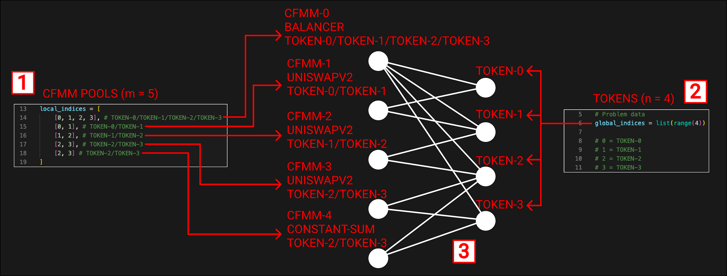
This looks complicated but I can assure you it isn’t.
The CFMM pools are declared in code as an array called “local_indices”. Each CFMM pool is itself an array where the items in the array determine which tokens are available within that pool. “m” is equal to 5 since we have 5 CFMM pools.
The tokens are declared in code as a list [ 0, 1, 2, 3 ] called “global indices”. “n” is equal to 4 since we have 4 items in the list. The numbers within this list represent tokens ie
0 = TOKEN-0
1 = TOKEN-1
While I have labeled these TOKEN-X for simplicity you can imagine these mapping to real tokens such as ETH, DAI, SOL etc.
The bipartite graph shows the CFMM pools on the left-hand side and the tokens on the right-hand side. A pool node is connected to a token node if that pool contains that token. This gives us a full representation of the network of CFMM pools we are working with.
Let’s quickly run through each CFMM.
CFMM 0 is a Balancer Pool (Balancer pools can hold more than 2 tokens)
[ 0, 1, 2, 3 ]
Contains TOKENS 0, 1, 2 & 3
CFMM 1 is a UniswapV2 Pool
[ 0, 1 ]
Contains TOKENS 0 & 1
CFMM 2 is a UniswapV2 Pool
[ 1, 2 ]
Contains TOKENS 1 & 2
CFMM 3 is a UniswapV2 Pool
[ 2, 3 ]
Contains TOKENS 2 & 3
CFMM 4 is a Constant-Sum Pool
[ 2, 3 ]
Contains TOKENS 2 & 3
At this point, you may be asking why the tokens were defined as “global_indices” and the CFMM pools as “local_indices”? Let’s find out.
Global vs Local Indices
The naming above refers to the global index labeling of tokens which applies to all CFMM pools and the local index labeling of tokens which applies to a specific CFMM pool.
To give you an example above we have declared the following global indexes.
0 → TOKEN-0
1 → TOKEN-1
2 → TOKEN-2
3 → TOKEN-3
If we look at the local index for CFMM-2 we have.
0 → TOKEN-1
1 → TOKEN-2
This means the index mapping of a token can be viewed globally or locally. If we look at the global index 0 we can see it maps to TOKEN-0. If we look at the local index 0 of CFMM-2 we can see it maps to TOKEN-1, a different token to the global index mapping.
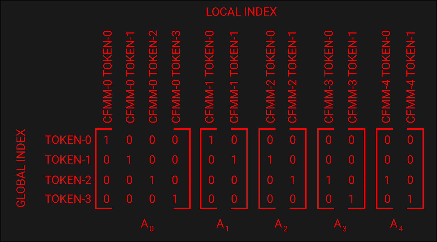
The local indices can be defined by the notation below,
Below is a table showing both the global index and local index of each CFMM.
Since our global index differs from our local ones we need to have a way of translating local indices to global indices.
Ultimately we want to see the net gain/loss of each token across the entire network of CFMM Pools after all trades have been completed. This will be viewed in the global index.
To do this translation from local index to global index a set of matrices is used.
Below is the set of Matrices for our example.
Note that A0 maps to CFMM-0, A1 to CFMM-1 etc. These matrices are generated using the following code.

We’ll see these matrices in action later in the article, for now, you just need to know they exist and that their purpose is mapping local indexes to global ones.
Next, we need to look at how we define our trades across the CFMMs.
Trades - Lambdas & Deltas
When making a trade/swap with a pool we have the amount we put into the pool, referred to as “Delta” and the amount we take out of the pool, known as “Lambda”.
Each token within the pool has its own “Delta” & “Lambda” values.
For example, if we traded against the UniswapV2 pool of ETH/DAI and put in 1 ETH and received 2000 DAI we would have the following values for “Delta” & “Lambda”.
ETH
Delta = 1
Lambda = 0
DAI
Delta = 0
Lambda = 2000
Trading Function
We can define the trade using “Delta” & “Lambda” and use those values to ensure the trade adheres to the trading function that governs the pool.
We define the trading function with the greek symbol phi φ.
Making a trade of “Delta i” & “Lambda i” against “CFMM i”
The trade results in converting the tendered tokens “Delta” into the received tokens “Lambda”
Trade is accepted if it meets the trading function constraint. The trading function phi takes in pool reserves, “Delta”, “Lambda” and “Gamma”.
“Gamma” represents the 1 minus the trading fee of the CFMM. This ensures we take into consideration the trading fee (0.3% for UniswapV2) that will be sent to the protocol from our “Delta” when we add tokens to the reserves.
The trading function ensures that the trade results in a new reserve that is greater than or equal to the trading function result of the old reserves.
Let’s see how we handle this in the code.
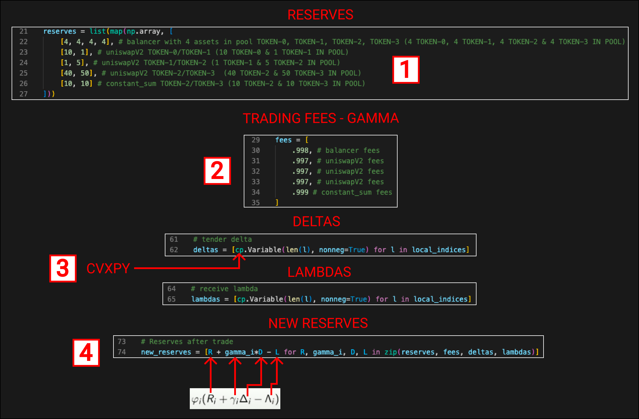
The reserves are declared for each CFMM pool. In this example these have been hardcoded, in reality, you would be constantly updating these reserves as trades happen on-chain. The first item in the array [ 4, 4, 4, 4 ] represents the Balancer pool and means we have the following within the pool
4 of TOKEN-0
4 of TOKEN-1
4 of TOKEN-2
4 of TOKEN-3
The trading fees are declared for each CFMM pool. The trading fees are defined as 1 - the actual fee. For example, UniswapV2 is a 0.3% fee so our fee is 0.997.
“Deltas” & “Lambdas” are declared and defined using cp which is the cvxpy library. This library is a convex optimisation solver. At this point in the code “Delta” & “Lambda” are abstract, they have no real value until we ask cvxpy to solve the optimisation.
The new reserves are declared. We can see they are calculated using the equation we saw earlier.
R = Reserves
gamma = “Gamma”
D = “Delta”
L = “Lambda”
Now we understand how each individual swap will be defined we can define the “Net Network Trade”.
Net Network Trade
The “Net Network Trade” is the +/- of each token in the network, at the end of all the trades, relative to our starting position.
This is where the “Ai” matrices we defined earlier will be used.
They allow us to take a trade against a CFMM pool which is made up of the tokens on that CFMM at their local indexes and combine it with our “Ai” matrix to update a global index array which will represent our “Net Network Trade”.
The “Net Network Trade” is represented by the greek letter psi Ψ. Its mathematical notation is seen below.
The image above states that psi Ψ is the sum of all trades across all CFMMs 1 → m where a trade is defined by “Lambda i” - “Delta i” and “Ai” is used to convert that trade into its global mapping.
Again let’s dive into the code, focusing on CFMM-2 as an example.
Psi is declared. Once again we’re using the cvxpy library. The @ symbol when used with matrices means the dot product of the 2 values. We have the A2 matrix which converts the local token indexes to global token indexes and (L-D) which is “Lambda” - “Delta” ie how much goes in during the swap and how much comes out. We sum the results for the CFMMs to give us our “Net Network Trade”.
Is a demonstration of the dot product method for those who aren’t familiar with matrix multiplication.
The result of the dot production calculation for CFMM-2 can be seen here. Each row represents the +/- of a token in the trade. Note the numbers above come from the cvxpy solution to our convex optimsation problem.
(0 * -0.224) + (0 * 0.931) = 0 = TOKEN-0
(1 * -0.224) + (0 * 0.931) = -0.224 = TOKEN-1
(0 * -0.224) + (1 * 0.931) = 0.931 = TOKEN-2
(0 * -0.224) + (0 * 0.931) = 0 = TOKEN-3
Above we have looked at CFMM-2 in isolation, now let’s look at the sum of all the CFMMs to get our “Net Network Trade” matrix.
Note, for this diagram we have rounded to 3 decimal places so the result will differ slightly from the python output in arbitrage.py.
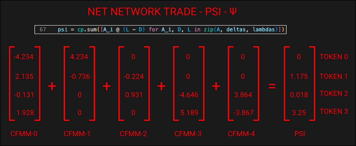
Each matrix represents the trade that occurred on that specific CFMM with positive values being received tokens and negative values being tendered tokens. By combining all these trades together we get our “Net Network Trade”.
CFMM-0 Executes a trade
Tenders 4.234 of TOKEN-0 & 0.131 of TOKEN-2
Receives 2.135 of TOKEN-1 & 1.928 of TOKEN-3
CFMM-1 Executes a trade
Tenders 0.736 of TOKEN-1
Receives 4.234 of TOKEN-0
CFMM-2 Executes a trade
Tenders 0.224 of TOKEN-1
Receives 0.931 of TOKEN-2
CFMM-3 Executes a trade
Tenders 4.646 of TOKEN-2
Receives 5.189 of TOKEN-3
CFMM-4 Executes a trade
Tenders 3.867 of TOKEN-3
Receives 3.864 of TOKEN-2
Net Network Trade
Receives 1.175 TOKEN-1, 0.018 TOKEN-2 & 3.25 TOKEN-3
Next, we need to think about what exactly it is we what to maximise. What is our objective function?
Objective (Utility) Function
The Objective Function sometimes known as the utility function is what we want to maximise.
So what do we want to maximise?
We want to maximise the total value we receive at the end of all the trades. To do this we can’t use the number of each individual token as token prices vary. We need to convert the tokens to a common unit of value, we need to normalise the data.
We can do this by getting the USD values of the tokens from external markets with deep liquidity.
This means our objective function is maximising the “Net Network Trade” in USD value. Let’s check out the code.
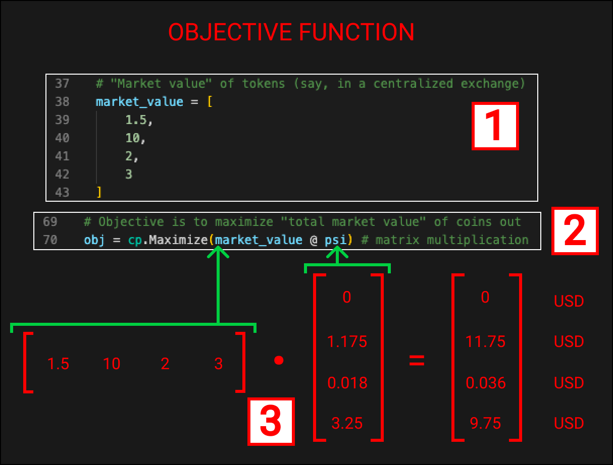
We define the market_value of each token. Here we use a hardcoded array but in reality, we would be constantly querying an exchange endpoint to get the latest prices.
$1.50 is the price for TOKEN-0
$10 is the price for TOKEN-1
etc.
The objective function is declared as obj. It states we want to maximise “market_value @ psi”, as I mentioned previously @ in this context means matrix multiplication.
These 2 matrices represent the market value and psi in the real solution. The resulting matrix is the “Net Network Trade” in USD value, exactly what we are trying to maximise.
As mentioned the values I’ve used here are from the actual solution, in reality prior to the convex optimisation being solved these are all abstract values.
I’ve included them as I feel seeing the real values rather than symbols can sometimes help with our understanding.
Note sometimes we may want to maximise the value for specific tokens. If we were only interested in acquiring TOKEN-0 & TOKEN-2 we could set the market value of TOKEN-1 & TOKEN-3 to zero. This will make the optimisation maximise the return value only in tokens 0 & 2 rather than across all 4 tokens.
We now have our objective function and can finally move on to the last piece of the puzzle, the constraints of the system.
Trading Constraints
The convex optimisation problem we have been setting up throughout the article exists within a network of CFMM pools.
These pools have their own laws that govern them.
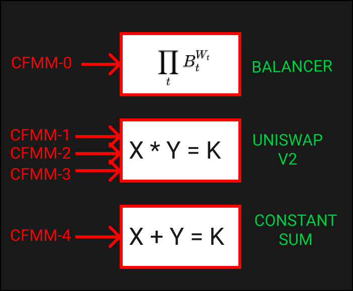
These laws come in the form of trading functions, which we touched on earlier. The most famous being Uniswaps “x * y = k”.
To dig into each CFMM’s trading function is outside the scope of this article but if you are interested have a read of this article.
Above are the trading functions for the 3 DEXs we are trading in. Within these 3 DEXs we are trading in 5 CFMM pools. Each pool has an arrow pointing to the trading function it uses.
Let’s see these constraints defined in the code.
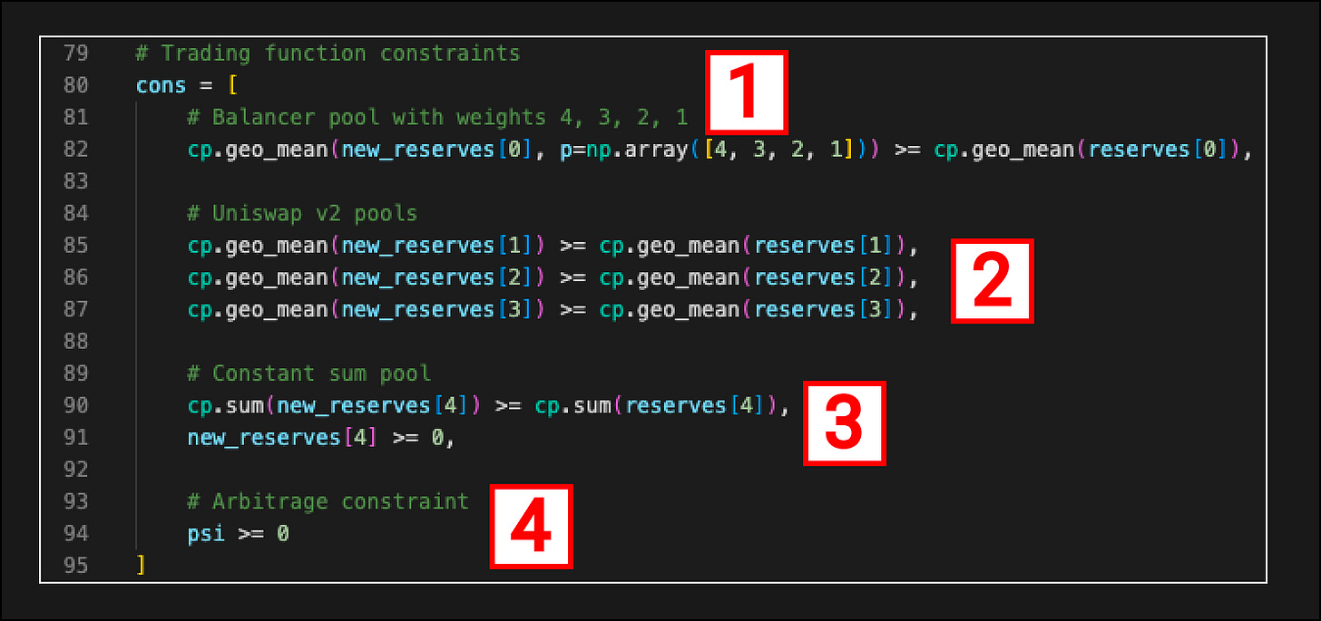
The Balancer trading function is a geometric mean function. It includes the weights of the tokens in the pool and is declared with the cp.geo_mean. The sum of the weights ( [ 4, 3, 2, 1 ] ) adds up to 1 representing all of the assets in the pool.
TOKEN-0 = 40%
TOKEN-1 = 30%
TOKEN-2 = 20%
TOKEN-3 = 10%
UniswapV2 is also a geometric mean market maker and so a cp.geo_mean can again be used to define the constraints for CFMM 1, 2 & 3.
Constant sum uses a different trading function and as such we use cp.sum.
This is not a trading function constraint but instead the constraint that turns our routing problem into an arbitrage problem that we discussed earlier.
By stating that at the end of all trades there should be no tokens that need to be tendered we turn the routing problem into an arbitrage problem.
This constraint checks that each token in psi (net network trade) is greater or equal to 0. This means at the end of all trades for every token we have either received that token or at least not had to tender any of that token.
Solving Convex Optimisation Problem
Now that we have our objective function and our constraints we can solve the convex optimisation problem.
The objective function and constraints, which effectively frame the problem, are displayed mathematically in Theo’s talk using the following notation.
Our Objective Function, which represents the “Net Network Trade” in USD
Our trading constraints for each CFMM from 1 → m
Valid values for trade amounts across all CFMMs (Note not explicitly defined in the code)
Arbitrage constraint, (cT)Ψ is our objective function where (cT) is the market values of the tokens. The arbitrage constraint is an indicator/penalty function. When Ψ >= 0 it will resolve to infinity otherwise it resolves to 0. Since anything where Ψ >= 0 will result in negative infinity, it ensures if this condition isn’t met that permutation won’t be selected (see Theo’s talk for more details).
The solution to the optimisation gives us the total value of the net network trade. By looking through the “Lambdas” & “Deltas” of each CFMM pool we can also see what trades were made to get to this result.
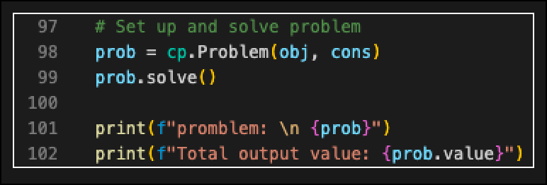
What cvxpy (cp) is doing under the hood to solve this problem would be another entire article so we’re not going to dive into it here. If you are interested I recommend starting here which is the documentation for CFMMRouter.jl, an optimiser written for this problem in julia.
For the context of this article what’s important is that we have a tool that solves convex optimistation problems and we now know how to programmatically frame questions we may want to ask.
After calling solve we will be given a list of trades that are known to be the trades that result in the optimal arbitrage. One issue we still have is that we don’t know in what order to execute them.
Execution Ordering
To kick-start an arbitrage some capital is required for the first trade (even if it is from a flashloan). As such our goal when ordering the trades should be to minimise the kick-start capital required.
Here we are going to minimise USD value across all the tokens to kick-start the trade. There may be situations where you have some of token x and so want to weight it towards that token.
The number of permutations for trade ordering is n! (n factorial) where n is the number of trades.
In our case we have 5 so we have 5 x 4 x 3 x 2 x 1 = 120 permutations.
To keep things simple we will brute force the trade orders to determine the best ordering.
The code is relatively simple and ultimately just loops through each permutation and keeps a tally of how much of each token was required taking into account any tokens that have been received in prior trades.
You can find the full arbitrage.py code below and play around with it yourself. I’ve added a few print statements and comments around the code to aid in your understanding.
| import numpy as np | |
| import cvxpy as cp | |
| import itertools | |
| # Problem data | |
| global_indices = list(range(4)) | |
| # 0 = TOKEN-0 | |
| # 1 = TOKEN-1 | |
| # 2 = TOKEN-2 | |
| # 3 = TOKEN-3 | |
| local_indices = [ | |
| [0, 1, 2, 3], # TOKEN-0/TOKEN-1/TOKEN-2/TOKEN-3 | |
| [0, 1], # TOKEN-0/TOKEN-1 | |
| [1, 2], # TOKEN-1/TOKEN-2 | |
| [2, 3], # TOKEN-2/TOKEN-3 | |
| [2, 3] # TOKEN-2/TOKEN-3 | |
| ] | |
| reserves = list(map(np.array, [ | |
| [4, 4, 4, 4], # balancer with 4 assets in pool TOKEN-0, TOKEN-1, TOKEN-2, TOKEN-3 (4 TOKEN-0, 4 TOKEN-1, 4 TOKEN-2 & 4 TOKEN-3 IN POOL) | |
| [10, 1], # uniswapV2 TOKEN-0/TOKEN-1 (10 TOKEN-0 & 1 TOKEN-1 IN POOL) | |
| [1, 5], # uniswapV2 TOKEN-1/TOKEN-2 (1 TOKEN-1 & 5 TOKEN-2 IN POOL) | |
| [40, 50], # uniswapV2 TOKEN-2/TOKEN-3 (40 TOKEN-2 & 50 TOKEN-3 IN POOL) | |
| [10, 10] # constant_sum TOKEN-2/TOKEN-3 (10 TOKEN-2 & 10 TOKEN-3 IN POOL) | |
| ])) | |
| fees = [ | |
| .998, # balancer fees | |
| .997, # uniswapV2 fees | |
| .997, # uniswapV2 fees | |
| .997, # uniswapV2 fees | |
| .999 # constant_sum fees | |
| ] | |
| # "Market value" of tokens (say, in a centralized exchange) | |
| market_value = [ | |
| 1.5, # TOKEN-0 | |
| 10, # TOKEN-1 | |
| 2, # TOKEN-2 | |
| 3 # TOKEN-3 | |
| ] | |
| # Build local-global matrices | |
| n = len(global_indices) | |
| m = len(local_indices) | |
| A = [] | |
| for l in local_indices: # for each CFMM | |
| n_i = len(l) # n_i = number of tokens avaiable for CFMM i | |
| A_i = np.zeros((n, n_i)) # Create matrix of 0's | |
| for i, idx in enumerate(l): | |
| A_i[idx, i] = 1 | |
| A.append(A_i) | |
| # Build variables | |
| # tender delta | |
| deltas = [cp.Variable(len(l), nonneg=True) for l in local_indices] | |
| # receive lambda | |
| lambdas = [cp.Variable(len(l), nonneg=True) for l in local_indices] | |
| psi = cp.sum([A_i @ (L - D) for A_i, D, L in zip(A, deltas, lambdas)]) | |
| # Objective is to maximize "total market value" of coins out | |
| obj = cp.Maximize(market_value @ psi) # matrix multiplication | |
| # Reserves after trade | |
| new_reserves = [R + gamma_i*D - L for R, gamma_i, D, L in zip(reserves, fees, deltas, lambdas)] | |
| # Trading function constraints | |
| cons = [ | |
| # Balancer pool with weights 4, 3, 2, 1 | |
| cp.geo_mean(new_reserves[0], p=np.array([4, 3, 2, 1])) >= cp.geo_mean(reserves[0]), | |
| # Uniswap v2 pools | |
| cp.geo_mean(new_reserves[1]) >= cp.geo_mean(reserves[1]), | |
| cp.geo_mean(new_reserves[2]) >= cp.geo_mean(reserves[2]), | |
| cp.geo_mean(new_reserves[3]) >= cp.geo_mean(reserves[3]), | |
| # Constant sum pool | |
| cp.sum(new_reserves[4]) >= cp.sum(reserves[4]), | |
| new_reserves[4] >= 0, | |
| # Arbitrage constraint | |
| psi >= 0 | |
| ] | |
| # Set up and solve problem | |
| prob = cp.Problem(obj, cons) | |
| prob.solve() | |
| # Trade Execution Ordering | |
| current_tokens = [0, 0, 0, 0] | |
| new_current_tokens = [0, 0, 0, 0] | |
| tokens_required_arr = [] | |
| tokens_required_value_arr = [] | |
| pool_names = ["BALANCER 0/1/2/3", "UNIV2 0/1", "UNIV2 1/2", "UNIV2 2/3", "CONSTANT SUM 2/3"] | |
| permutations = itertools.permutations(list(range(len(local_indices))), len(local_indices)) | |
| permutations2 = [] | |
| for permutation in permutations: | |
| permutations2.append(permutation) | |
| current_tokens = [0, 0, 0, 0] | |
| new_current_tokens = [0, 0, 0, 0] | |
| tokens_required = [0, 0, 0, 0] | |
| for pool_id in permutation: | |
| pool = local_indices[pool_id] | |
| for global_token_id in pool: | |
| local_token_index = pool.index(global_token_id) | |
| new_current_tokens[global_token_id] = current_tokens[global_token_id] + (lambdas[pool_id].value[local_token_index] - deltas[pool_id].value[local_token_index]) | |
| if new_current_tokens[global_token_id] < 0 and new_current_tokens[global_token_id] < current_tokens[global_token_id]: | |
| if current_tokens[global_token_id] < 0: | |
| tokens_required[global_token_id] += (current_tokens[global_token_id] - new_current_tokens[global_token_id]) | |
| new_current_tokens[global_token_id] = 0 | |
| else: | |
| tokens_required[global_token_id] += (-new_current_tokens[global_token_id]) | |
| new_current_tokens[global_token_id] = 0 | |
| current_tokens[global_token_id] = new_current_tokens[global_token_id] | |
| tokens_required_value = [] | |
| for i1, i2 in zip(tokens_required, market_value): | |
| tokens_required_value.append(i1*i2) | |
| tokens_required_arr.append(tokens_required) | |
| tokens_required_value_arr.append(sum(tokens_required_value)) | |
| min_value = min(tokens_required_value_arr) | |
| min_value_index = tokens_required_value_arr.index(min_value) | |
| print("\n-------------------- ARBITRAGE TRADES + EXECUTION ORDER --------------------\n") | |
| for pool_id in permutations2[min_value_index]: | |
| pool = local_indices[pool_id] | |
| print(f"\nTRADE POOL = {pool_names[pool_id]}") | |
| for global_token_id in pool: | |
| local_token_index = pool.index(global_token_id) | |
| if (lambdas[pool_id].value[local_token_index] - deltas[pool_id].value[local_token_index]) < 0: | |
| print(f"\tTENDERING {-(lambdas[pool_id].value[local_token_index] - deltas[pool_id].value[local_token_index])} TOKEN {global_token_id}") | |
| for global_token_id in pool: | |
| local_token_index = pool.index(global_token_id) | |
| if (lambdas[pool_id].value[local_token_index] - deltas[pool_id].value[local_token_index]) >= 0: | |
| print(f"\tRECEIVEING {(lambdas[pool_id].value[local_token_index] - deltas[pool_id].value[local_token_index])} TOKEN {global_token_id}") | |
| print("\n-------------------- REQUIRED TOKENS TO KICK-START ARBITRAGE --------------------\n") | |
| print(f"TOKEN-0 = {tokens_required_arr[min_value_index][0]}") | |
| print(f"TOKEN-1 = {tokens_required_arr[min_value_index][1]}") | |
| print(f"TOKEN-2 = {tokens_required_arr[min_value_index][2]}") | |
| print(f"TOKEN-3 = {tokens_required_arr[min_value_index][3]}") | |
| print(f"\nUSD VALUE REQUIRED = ${min_value}") | |
| print("\n-------------------- TOKENS & VALUE RECEIVED FROM ARBITRAGE --------------------\n") | |
| net_network_trade_tokens = [0, 0, 0, 0] | |
| net_network_trade_value = [0, 0, 0, 0] | |
| for pool_id in permutations2[min_value_index]: | |
| pool = local_indices[pool_id] | |
| for global_token_id in pool: | |
| local_token_index = pool.index(global_token_id) | |
| net_network_trade_tokens[global_token_id] += lambdas[pool_id].value[local_token_index] | |
| net_network_trade_tokens[global_token_id] -= deltas[pool_id].value[local_token_index] | |
| for i in range(0, len(net_network_trade_tokens)): | |
| net_network_trade_value[i] = net_network_trade_tokens[i] * market_value[i] | |
| print(f"RECEIVED {net_network_trade_tokens[0]} TOKEN-0 = ${net_network_trade_value[0]}") | |
| print(f"RECEIVED {net_network_trade_tokens[1]} TOKEN-1 = ${net_network_trade_value[1]}") | |
| print(f"RECEIVED {net_network_trade_tokens[2]} TOKEN-2 = ${net_network_trade_value[2]}") | |
| print(f"RECEIVED {net_network_trade_tokens[3]} TOKEN-3 = ${net_network_trade_value[3]}") | |
| print(f"\nSUM OF RECEIVED TOKENS USD VALUE = ${sum(net_network_trade_value)}") | |
| print(f"CONVEX OPTIMISATION SOLVER RESULT: ${prob.value}\n") |
Here is the output from the code defining the trades, their execution order, the minimum number of tokens required to kick start the trade and the total tokens received from the arbitrage.
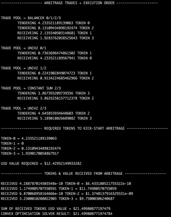
There we have it I hope you’ve learned something new and added a new tool to your arbitrage tool kit.
Til next time
noxx
Follow me on Twitter @noxx3xxon





Thanks this is very well written. Any reason why you would approach it as an optimization problem rather than a graph problem?
Currently working in risk analysis on tradFI (I'm a mathematician). Is convex opt. a way into a position in DeFi? Engineer or analyst, doesn't matter.